

Analysis of Pendulum-cart system and newtonian physics.
In modern Newtonian physics reside two of the most important and widely used mechanical systems; that is, pendulums and springs. Nowadays these systems are ubiquitous in our modern world, appearing in a vast number of mechanical systems such as clocks, car suspensions, metronomes, mattresses, and shock absorbers. The influence these two mechanical systems have had in our everyday life motivates their further study. Thus, B.R.I.T decided to study and model a pendulum-cart mechanism by utilizing equations of motion, free body diagrams, differential equations, and python for a numerical and graphical solution of the system.
Content
- 5) Conclusion
1. What is a pendulum-cart system
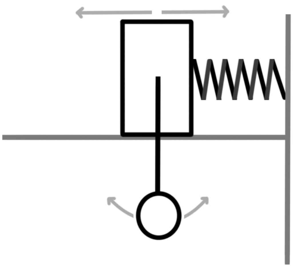
A pendulum-cart system consists of a cart moving in a horizontal trajectory while being attached to a spring on a wall. Thus, converting the cart’s linear motion into a back-and-forth pattern like that of a simple harmonic oscillator. Additionally, a pendulum is suspended from the cart which will move in response to the cart’s motion.
1.1 Axis and parameter set up
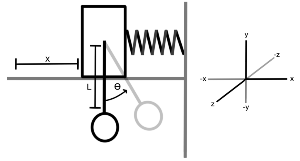
Before we can analyse the system, certain parameters and axis must be chosen. To simplify things, an < 𝑥, 𝑦, 𝑧 > axis was chosen such that the diagram looks as follows. Here, ‘𝑧’ is an important axis because of the torque’s direction.
- X = position of the cart (m)
- L = Length of the pendulum rod (m)
- ϴ = Angle of pendulum (rad)
1.2 Free-body diagram
To further our understanding of the system, we will determine all forces acting on it by creating a free-body diagram to both the pendulum and the cart.
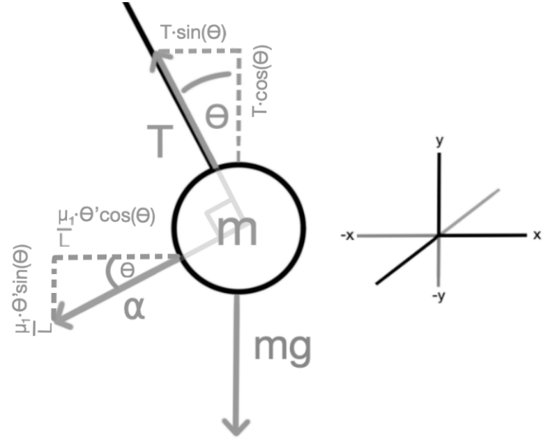
Free-body diagram for the pendulum
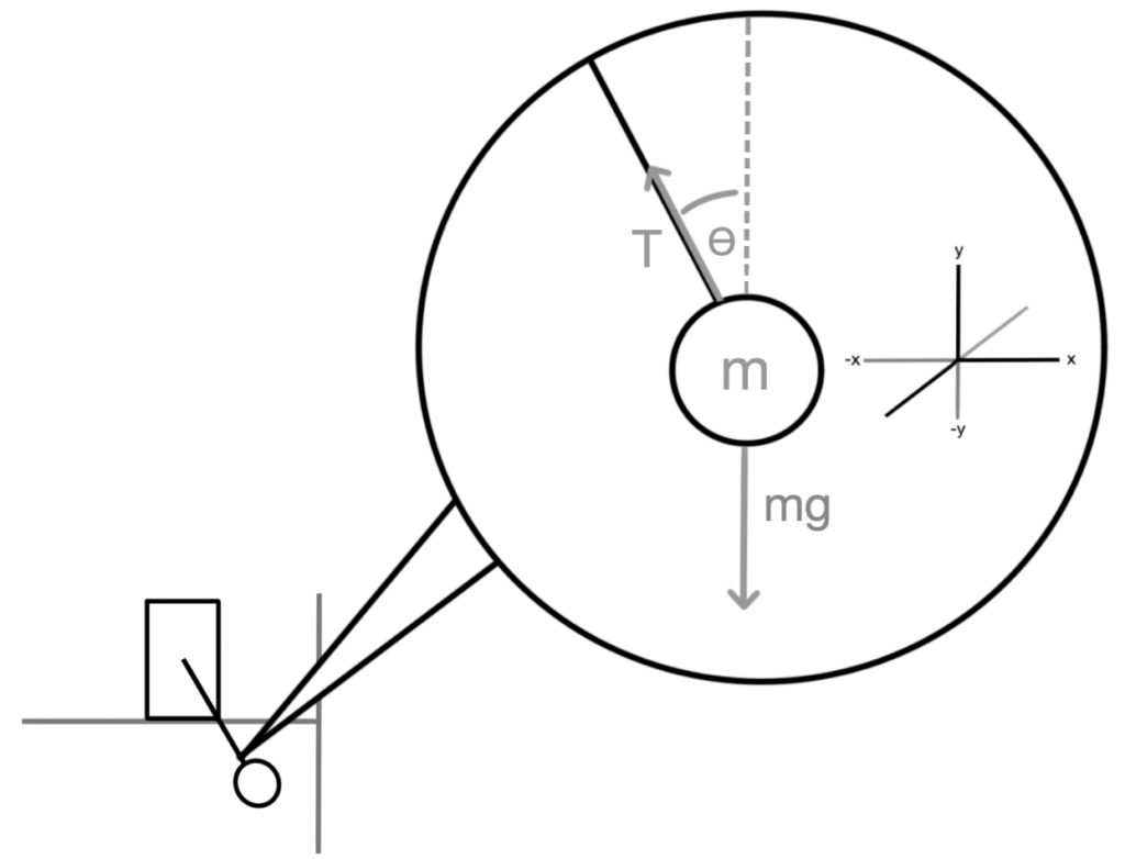
m = mass of pendulum (kg)
g = gravitational constant (9.8m/s2)
μ1 = friction coefficient pendulum
T = tension (N)
⍺ = friction force (N)
mg = force due to gravity (N)
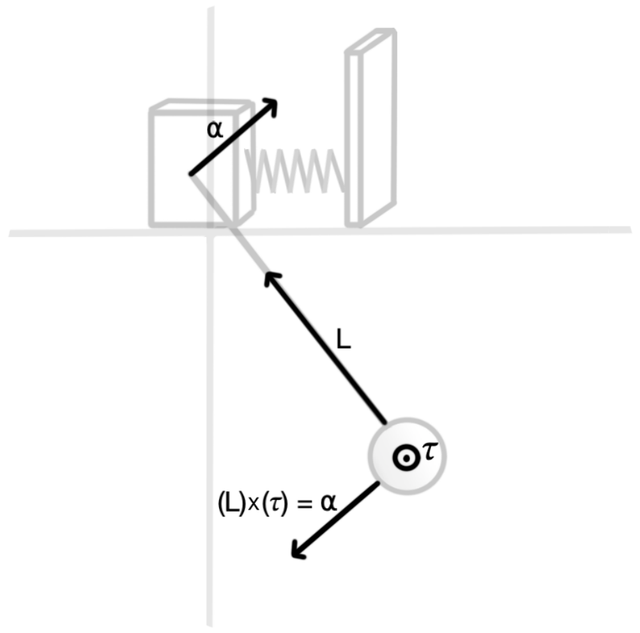
the force that creates the torque ‘𝜏’ can be represented as a force ‘⍺’ acting on both the pendulum and the cart (because of newtons 3rd law). If we take into consideration this new force ‘⍺’ and the length of the rod ‘L’ as a vector, then we could find the torque by computing a cross product between them.
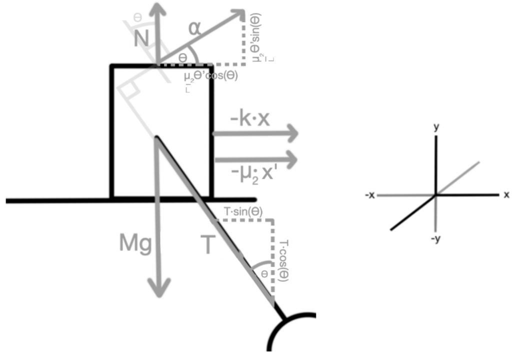
Free-body diagram for the cart
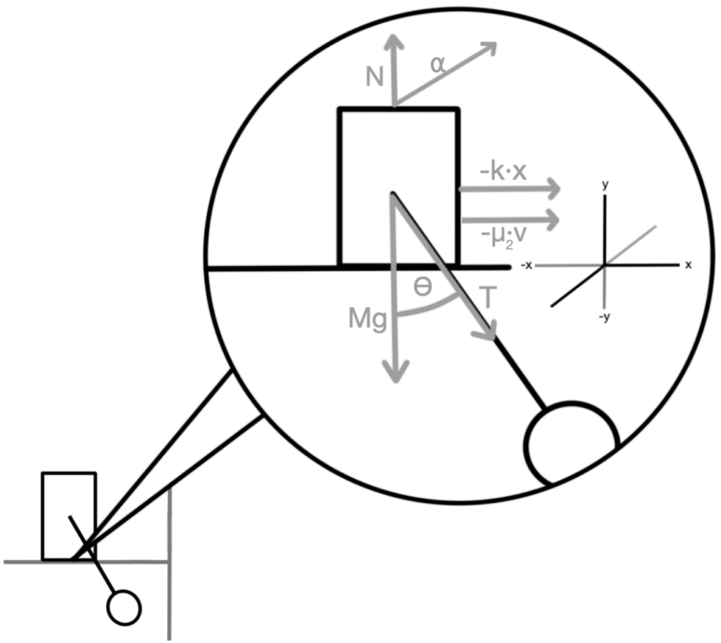
M = mass of the cart (kg)
g = gravitational constant (9.8m/s2)
μ2 = friction coefficient cart
v = velocity (m/s)
k = Spring constant (N/m)
T = tension (N)
⍺ = friction force (N)
mg = force due to gravity (N)
N = normal force (N)
2. Newton’s second law for the pendulum
Applying Newton’s second law will allow us to further examine the mechanics of the system. However, one must first establish certain mathematical relationship between the cart and the pendulum’s position. To do so, we will relate the cart’s position ‘𝑥’ with the pendulum’s position in both < 𝑥, 𝑦, 0 > direction which we will call ‘𝑋 ’ and ‘𝑌 ’ respectively. Ultimately, this relationship will allow us to relate their second derivative with Newton’s second law.
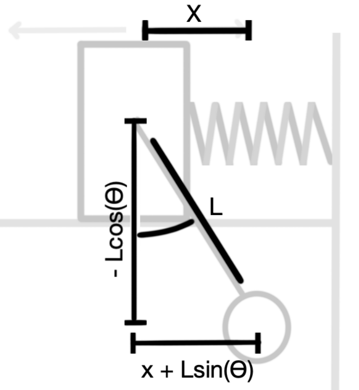
𝑥𝑝 = 𝑥 + 𝐿𝑠𝑖𝑛(𝜃)
𝑌p = −𝐿𝑐𝑜𝑠(𝜃)
𝑥′𝑝 = 𝑥′ + 𝜃′𝐿𝑐𝑜𝑠(𝜃)
𝑌′𝑝 = 𝜃′𝐿𝑠𝑖𝑛(𝜃)
𝑥′′𝑝 = 𝑥′′ + 𝐿[𝜃′′ cos(𝜃) − (𝜃′)2 sin(𝜃)]
𝑌′′𝑝 = 𝜃′′𝐿𝑠𝑖𝑛(𝜃) + (𝜃′)2Lcos (𝜃)
Newton’s second law states that the force is equal to the mass times its acceleration.
Thus, in the < 𝑥, 0,0 > direction we have the following equation.
∑𝐹𝑜𝑟𝑐𝑒𝑠𝑥 𝑝𝑒𝑛𝑑𝑢𝑙𝑢𝑚 = 𝑚𝑎𝑠𝑠∙𝑎𝑐𝑐𝑒𝑙𝑒𝑟𝑎𝑡𝑖𝑜𝑛x
−𝑇𝑠𝑖𝑛(𝜃) − 1/L[𝜇1 𝜔cos (𝜃)] = 𝑚 ∙ 𝑥′′
i) −𝑇𝑠𝑖𝑛(𝜃) − 1/L[𝜇1 𝜃′cos (𝜃)] = 𝑚 ∙ [𝑥′′ + 𝐿(𝜃′′ cos(𝜃) − (𝜃′)2 sin(𝜃))]
∑𝐹𝑜𝑟𝑐𝑒𝑠𝑦 𝑝𝑒𝑛𝑑𝑢𝑙𝑢𝑚 =𝑚𝑎𝑠𝑠∙𝑎𝑐𝑐𝑒𝑙𝑒𝑟𝑎𝑡𝑖𝑜𝑛𝑦
𝑡𝑐𝑜𝑠(𝜃) − 𝑚𝑔 − 1/L[𝜇1 𝜔𝑠𝑖𝑛 (𝜃)] = 𝑚 ∙ 𝑦′′
ii) 𝑇𝑐𝑜𝑠(𝜃) − 𝑚𝑔 − 1/L[(𝜇1)𝜃′ 𝑠𝑖𝑛(𝜃)] = 𝑚 ∙ [𝜃′′𝐿𝑠𝑖𝑛(𝜃) + 𝐿(𝜃′)2cos (𝜃)]
2.1 Newton’s second law for the cart
Here, we will follow the same steps as before, but this time will apply them to the cart. This will give us the equations of motion for the cart. Clearly, the cart will have no acceleration on < 0, 𝑦, 0 > direction.
∑𝐹𝑜𝑟𝑐𝑒𝑠𝑥 𝑐𝑎𝑟𝑡 = 𝑚𝑎𝑠𝑠∙𝑎𝑐𝑐𝑒𝑙𝑒𝑟𝑎𝑡𝑖𝑜𝑛𝑥
−𝑘𝑥 − 𝜇2𝑣 + 𝑇𝑠𝑖𝑛(𝜃) + 1/L[𝜇1 𝜔cos (𝜃)] = M ∙ 𝑥′′
iii) 𝑇𝑠𝑖𝑛(𝜃) + 1/L[𝜇1𝜃′cos(𝜃)] − 𝑘𝑥 − 𝜇2𝑥′ = 𝑀∙𝑥′′
∑𝐹𝑜𝑟𝑐𝑒𝑠𝑦 𝑐𝑎𝑟𝑡 =𝑚𝑎𝑠𝑠∙𝑎𝑐𝑐𝑒𝑙𝑒𝑟𝑎𝑡𝑖𝑜𝑛𝑦
𝑁 + (𝜇1 𝜃′cos (𝜃))/L − 𝑀𝑔 − 𝑇𝑐𝑜𝑠(𝜃) = 0
3. Equations of motion
Clearly, there are three main equations derived from Newton’s second law. There are two equations from the pendulum ‘i)’ and ‘ii)’, and only one equation from the cart ‘iii)’ since the cart has no acceleration in the < 0, 𝑦, 0 > direction.
i) −𝑇𝑠𝑖𝑛(𝜃) − 1/L[𝜇1 𝜃′cos (𝜃)] = 𝑚 ∙ [𝑥′′ + 𝐿(𝜃′′ cos(𝜃) − (𝜃′)2 sin(𝜃))]
ii) 𝑇𝑐𝑜𝑠(𝜃) − 𝑚𝑔 − 1/L[(𝜇1)𝜃′ 𝑠𝑖𝑛(𝜃)] = 𝑚 ∙ [𝜃′′𝐿𝑠𝑖𝑛(𝜃) + 𝐿(𝜃′)2cos (𝜃)]
iii) 𝑇𝑠𝑖𝑛(𝜃) + 1/L[𝜇1𝜃′cos(𝜃)] − 𝑘𝑥 − 𝜇2𝑥′ = 𝑀∙𝑥′′
If we were to add equation ‘i)’ and ‘iii)’ together we would be creating, and simplifying, a new equation which we will call ‘iv)’ as such.
−𝑇𝑠𝑖𝑛(𝜃) − 1/L[𝜇1 𝜃′cos (𝜃)] + 𝑇𝑠𝑖𝑛(𝜃) + 1/L[𝜇1𝜃′cos(𝜃)]− 𝑘𝑥 − 𝜇2𝑥′ = [ 𝑚 ∙ [𝑥′′ + 𝐿(𝜃′′ cos(𝜃) − (𝜃′)2 sin(𝜃))] ] + [𝑀∙𝑥′′]
− 𝑘𝑥 − 𝜇2𝑥′ = 𝑥′′ (m + M) + Lm(𝜃′′ cos(𝜃) – (𝜃′)2 sin(𝜃))
iv) 𝑥′′ (m + M)+ 𝑘𝑥 + 𝜇2𝑥′ = Lm((𝜃′)2 sin(𝜃) – 𝜃′′ cos(𝜃))
This new equation ‘iv)’ is particularly useful because it removes the unknown tension ‘T’ from one of the equations. Thus, leaving us with the following two formulas.
ii) 𝑇𝑐𝑜𝑠(𝜃) − 𝑚𝑔 − 1/L[(𝜇1)𝜃′ 𝑠𝑖𝑛(𝜃)] = 𝑚 ∙ [𝜃′′𝐿𝑠𝑖𝑛(𝜃) + 𝐿(𝜃′)2cos (𝜃)]
iv) 𝑥′′ (m + M)+ 𝑘𝑥 + 𝜇2𝑥′ = Lm((𝜃′)2 sin(𝜃) – 𝜃′′ cos(𝜃))
However, we still have tension ‘𝑇’ as an unknown variable in equation ‘𝑖𝑖)’. To get rid of it, one can multiply ‘i)’ by cos (𝜃) and ‘ii)’ by sin (𝜃) and add them together, we will call this new equation ‘v)’.
[i)∙cos(θ)]
−𝑇𝑠𝑖𝑛(𝜃)cos (𝜃) − 1/L[𝜇1 𝜃′cos2(𝜃)] = 𝑚𝑥′′cos (𝜃) + 𝐿𝑚𝜃′′ cos2(𝜃) − 𝐿𝑚(𝜃′)2 sin(𝜃) cos (𝜃)
[ii)∙sin(θ)]
𝑇𝑠𝑖𝑛(𝜃)𝑐𝑜𝑠(𝜃) − 𝑚𝑔 ∙ sin (𝜃) − 1/L[𝜇1 𝜃′ 𝑠𝑖𝑛2(𝜃)] = 𝐿𝑚𝜃′′𝑠𝑖𝑛2(𝜃) + 𝐿𝑚(𝜃′)2sin (𝜃)cos (𝜃)
[i)∙cos(θ)]+ [ii)∙ sin(θ)]
− 1/L[𝜇1]𝜃′(𝑠𝑖𝑛2(𝜃) + cos2(𝜃)) − 𝑚𝑔 ∙ sin(𝜃) = 𝐿𝑚𝜃′′[𝑠𝑖𝑛2(𝜃) + cos2(𝜃)] + 𝑚𝑥′′ cos(𝜃)
v) −1/L𝜇1 𝜃′ − 𝑚𝑔 ∙ sin(𝜃) = 𝐿𝑚𝜃′′ + 𝑚𝑥′′ cos(𝜃)
Finally, we are left with two equations without the tension variable ‘𝑇’.
iv) 𝑥′′(𝑚 + 𝑀) + 𝑘𝑥 + 𝜇2𝑥′ = 𝐿𝑚[(𝜃′)2 sin(𝜃) − 𝜃′′ cos(𝜃)]
v) −1/L𝜇1 𝜃′ − 𝑚𝑔 ∙ sin(𝜃) = 𝐿𝑚𝜃′′ + 𝑚𝑥′′ cos(𝜃)
3.1 Solving second derivative in terms of lower derivative variables
Clearly, ‘iv)’ and ‘v)’ are equations in terms of first and second derivatives of the angle and position. However, before we can transform them as two first order DE’s, we would first need to write 𝜃′′ and 𝑥′′ in terms of lower derivative variables that is 𝜃, 𝜃′ and 𝑥, 𝑥′. To do so, we need to multiply equation ‘v)’ by cos (θ) and add equation ‘iv)’ thereby eliminating 𝜃′′ from the equation. Then, solving for 𝑥’’ will input a new equation which we will call ‘vi)’.
[v)∙cos(θ)]
− 1/L[𝜇1 𝜃′cos (𝜃)] − 𝑚𝑔 ∙ sin(𝜃)cos (𝜃) = 𝐿𝑚𝜃′′cos (𝜃) + 𝑚𝑥′′ cos2(𝜃)
[v)∙cos(θ)]+[iv)]
𝑥′′(𝑚 + 𝑀) + 𝑘𝑥 + 𝜇2𝑥′ − 1/L[𝜇1 𝜃′ cos(𝜃)] − 𝑚𝑔 ∙ sin(𝜃) cos(𝜃) = 𝑚𝑥′′ cos2(𝜃) + 𝐿𝑚(𝜃′)2 sin(𝜃)
𝑥′′(𝑚 + 𝑀) − 𝑚𝑥′′ cos2(𝜃) = 𝐿𝑚(𝜃′)2sin(𝜃) + 𝑚𝑔 ∙ sin(𝜃)cos(𝜃) + 1/L[𝜇1 𝜃′ cos(𝜃)] − 𝑘𝑥 − 𝜇2𝑥′
𝑥′′[(𝑚 + 𝑀) − 𝑚 cos2(𝜃)] = 𝐿𝑚(𝜃′)2 sin(𝜃) + 𝑚𝑔 ∙ sin(𝜃) cos(𝜃) + 1/L[𝜇1 𝜃′ cos(𝜃)] − 𝑘𝑥 − 𝜇2𝑥′
𝑥′′ = [ 𝐿𝑚(𝜃′)2 sin(𝜃) + 𝑚𝑔 ∙ sin(𝜃) cos(𝜃) + 1/L[𝜇1 𝜃′ cos(𝜃)] − 𝑘𝑥 − 𝜇2𝑥′ ] / [ (𝑚 + 𝑀) − 𝑚 cos2(𝜃) ]
𝑥′′ = [ 𝐿𝑚(𝜃′)2 sin(𝜃) + 𝑚𝑔 ∙ sin(𝜃) cos(𝜃) + 1/L[𝜇1 𝜃′ cos(𝜃)] − 𝑘𝑥 − 𝜇2𝑥′ ] / [(𝑚 + 𝑀) − 𝑚 (1 + sin2(𝜃))]
𝑥′′ = [ 𝐿𝑚(𝜃′)2 sin(𝜃) + 𝑚𝑔 ∙ sin(𝜃) cos(𝜃) + 1/L[ 𝜇1 𝜃′ cos(𝜃)] − 𝑘𝑥 − 𝜇2𝑥′ ] / [𝑀 + m ∙ sin2(𝜃)]
Now, we can multiply equation ‘v)’ by (𝑚 + 𝑀) and multiply equation ‘iv)’ by 𝑚 ∙ cos (𝜃) and add them together thereby allowing the isolation of 𝜃′′ in one single equation which we will call ‘vii)’.
[v)∙(m+M)]
(𝑚+𝑀)∙1/L[−𝜇1𝜃′ −𝑚𝑔∙sin(𝜃)] = (𝑚+𝑀)𝐿𝑚𝜃′′ +𝑚𝑥′′(𝑚+𝑀)cos(𝜃)
[iv) ∙ mcos(θ)]
𝑚𝑥′′(𝑚 + 𝑀)cos (𝜃) + 𝑘𝑥𝑚cos (𝜃) + 𝜇2𝑥′cos (𝜃) = 𝐿𝑚2(𝜃′)2 sin(𝜃)cos (𝜃) − 𝐿𝑚2𝜃′′ cos2(𝜃)
[v)∙(m+M)] + [iv)∙mcos(θ)]
−(𝑚 + 𝑀)1/L( 𝜇1 𝜃′) − (𝑚 + 𝑀)𝑚𝑔 ∙ sin(𝜃) + 𝑘𝑥𝑚 cos(𝜃) + 𝜇2𝑥′cos (𝜃) = (𝑚 + 𝑀)𝐿𝑚𝜃′′ + 𝐿𝑚2(𝜃′)2 sin(𝜃)cos (𝜃) − 𝐿𝑚2𝜃′′ cos2(𝜃)
−(𝑚 + 𝑀)1/L( 𝜇1 𝜃′) − (𝑚 + 𝑀)𝑚𝑔 ∙ sin(𝜃) + 𝑘𝑥𝑚 cos(𝜃) + 𝜇2𝑥′cos (𝜃) – 𝐿𝑚2(𝜃′)2 sin(𝜃)cos (𝜃) = (𝑚 + 𝑀)𝐿𝑚𝜃′′− 𝐿𝑚2𝜃′′ cos2(𝜃)
−(𝑚 + 𝑀)1/L( 𝜇1 𝜃′) − (𝑚 + 𝑀)𝑚𝑔 ∙ sin(𝜃) + 𝑘𝑥𝑚 cos(𝜃) + 𝜇2𝑥′cos (𝜃) – 𝐿𝑚2(𝜃′)2 sin(𝜃)cos (𝜃) / (𝑚 + 𝑀)𝐿𝑚− 𝐿𝑚2cos2(𝜃) = 𝜃′′
−(𝑚 + 𝑀)1/L( 𝜇1 𝜃′) − (𝑚 + 𝑀)𝑚𝑔 ∙ sin(𝜃) + 𝑘𝑥𝑚 cos(𝜃) + 𝜇2𝑥′cos (𝜃) – 𝐿𝑚2(𝜃′)2 sin(𝜃)cos (𝜃) / (𝑚 + 𝑀)𝐿𝑚− 𝐿𝑚2(1-sin2(𝜃)) = 𝜃′′
−(1 + 𝑀/m)1/L( 𝜇1 𝜃′) − (𝑚 + 𝑀)𝑔 ∙ sin(𝜃) + 𝑘𝑥 cos(𝜃) + 𝜇2𝑥′cos (𝜃) – 𝐿𝑚(𝜃′)2 sin(𝜃)cos (𝜃) / L(M+msin2(𝜃)) = 𝜃′′
− (𝑚 + 𝑀)𝑔∙ sin(𝜃) – 𝐿𝑚(𝜃′)2 sin(𝜃)cos (𝜃 − (1 + 𝑀/m)1/L( 𝜇1 𝜃′) + cos(𝜃)∙[𝑘𝑥 + 𝜇2𝑥′] / L(M+msin2(𝜃)) = 𝜃′′
Now, we have two single variable-independent equations ‘vi)’ and ‘vii)’
vi) 𝑥′′ = [ 𝐿𝑚(𝜃′)2 sin(𝜃) + 𝑚𝑔 ∙ sin(𝜃) cos(𝜃) + 1/L[ 𝜇1 𝜃′ cos(𝜃)] − 𝑘𝑥 − 𝜇2𝑥′ ] / [𝑀 + m ∙ sin2(𝜃)]
vii) 𝜃′′ = − (𝑚 + 𝑀)𝑔∙ sin(𝜃) – 𝐿𝑚(𝜃′)2 sin(𝜃)cos (𝜃 − (1 + 𝑀/m)1/L( 𝜇1 𝜃′) + cos(𝜃)∙[𝑘𝑥 + 𝜇2𝑥′] / L(M+msin2(𝜃))
3.2 First order DE transformation
Now that we have two equations in terms of lower derivative variables, we can re-write them as two first order differential equations which is essential if we want to solve them numerically using 𝑅𝑢𝑛𝑔𝑒 𝐾𝑢𝑡𝑡𝑎 methods. Thus, we would need to re-write the variables as such:
𝑥′ = 𝑣
𝜃′ = 𝜔
𝑣′ = [ 𝐿𝑚𝜔2sin(𝜃) + 𝑚𝑔∙sin(𝜃)cos(𝜃) + 1/L(𝜇1𝜔cos(𝜃))−𝑘𝑥−𝜇2𝑣) ] / [ 𝑀 + m∙sin2(𝜃) ]
𝜔’ = [ −(𝑚+𝑀)𝑔∙sin(𝜃) − 𝐿𝑚𝜔2sin(𝜃)cos(𝜃) − (1+𝑀)(1/L)𝜇1𝜔 + cos(𝜃)[𝑘𝑥 + 𝜇 𝑣] ] / [𝐿(𝑀 + 𝑚𝑠𝑖𝑛2(𝜃))]
This method of re-writing is particularly useful when coding in python because we will be able to assign variables 𝑥, 𝜃, 𝑣, 𝑤, 𝑣′, 𝑤′, which are functions, to each component of the mechanical system; that is the cart and the pendulum.
4. Mechanical System in Python
Before we can model the system in python, we will import the necessary libraries which will allows us to use trigonometric functions, lines, etc.
import numpy as np                            # necessary libraries
import matplotlib.pyplot as plt
import scipy.integrate as integrate
import matplotlib.animation as animation
Similarly, we will need to choose certain parameters for our mechanical system. These will be the default parameters for all scenarios studied below.
M = 5     # Mass of the cart
m = 0.1   # mass of the pendulum
k = 25    # spring constant
L = 0.5   # lenght of string
g = 9.8   # gravitational acceleration
u1 = 0.1  # friction coefficient pendulum
u2 = 20   # friction coefficient cart
Then, we will need to assign the derivatives of our equations ‘𝑣𝑖)’ and ‘𝑣𝑖𝑖)’ certain states. Here, clearly:
𝑑𝑒𝑟[0] = 𝑥′ 𝑠𝑡𝑎𝑡𝑒 [1] = 𝑣 𝑑𝑒𝑟[2] = 𝜃′ 𝑠𝑡𝑎𝑡𝑒[3] = 𝜔
As explained above, this is the way we’re writing our four equations in python.
def der_state(t, state):                                          # Here, we are writing first order DE.
        """compute the derivative of the given state"""

        der = np.zeros_like(state)
        der[0] = state[1]           #    state[0] = x
        der[2] = state[3]           #    state[2] = theta
        der[1] = ((((L*m)*state[3]**2)*np.sin(state[2])) + m*g*np.sin(state[2])*np.cos(state[2]) + (u1/L)*state[3]*np.cos(state[2]) - k*state[0] - u2*state[1])/(M + m*np.sin(state[2])*np.sin(state[2]))
        der[3] = (-(m + M)*g*np.sin(state[2]) - (L*m)*(state[3]**2)*np.sin(state[2])*np.cos(state[2]) - (1 + (M/m))*(u1/L)*state[3] + np.cos(state[2])*(k*state[0] + u2*state[1]))/(L*M + L*m*np.sin(state[2])*np.sin(state[2]))
        return der
Similarly, we will need to choose an initial condition. Otherwise, neither the cart nor the pendulum will have motion. We will choose an initial condition on the cart and on the angle of the pendulum.
state0 = ([1, 0, 1, 0]) # [x],[x'],[theta],[theta'] initial conditionsThe following code was used to solve the differential equations above. Then, the following set of code is used to define the cartesian coordinates so that we can plot on the graph.
sol = integrate.solve_ivp(der_state, (0, tf), state0, t_eval=T)     #this solves both previous DE.
ang_pendulum_pos = sol.y[2]
x_quisite_position_cart = sol.y[0]

# Cartesian coordinates
x2 = x_quisite_position_cart
y2 = 0 # no motion in y direction.

x = x2 + L*np.sin(ang_pendulum_pos)
y = -L*np.cos(ang_pendulum_pos) #the y-axis points down
We will also import another library from matplotlib which will let us display the animation on our screen. We will set up an axis, provide limits, and the type of grid as follows:
from matplotlib import rc
rc('animation', html='html5')

fig = plt.figure()
ax = fig.add_subplot(111, autoscale_on=False, xlim=(-2, 2.1), ylim=(-1, 1))       # setting the graph axis
ax.grid()
Finally, we will define all our objects (cart, pendulum, lines, table, wall, spring), we will assign them colors, width, size, type of lines (using matplotlib libraries). All of these are explained in the full code provided. Thus, giving us something that looks like this:
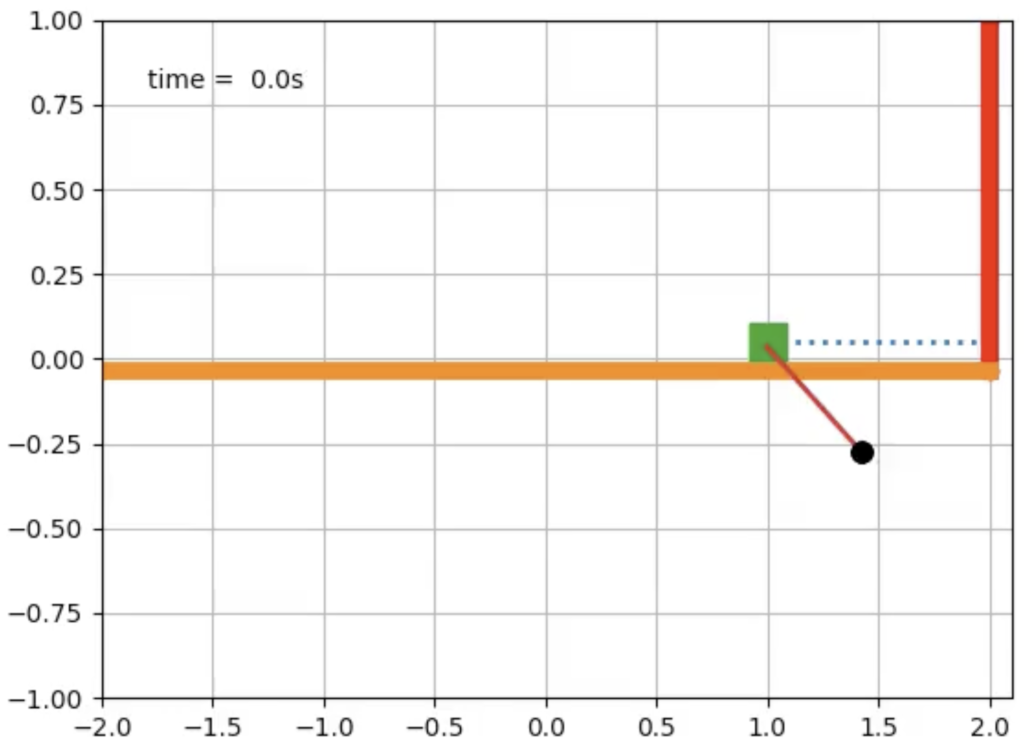
4.1 Evaluating certain scenarios
Now, we have a working mechanical system in python.
https://colab.research.google.com/
Thus, we will start the evaluation of certain scenarios. In total we will study three main scenarios plus two interesting cases, these being:
- Over damped system
- Underdamped system
- Critically damped system
- System under Moon’s gravity
- System with heavy pendulum
Scenario #1
The system is overdamped. For this scenario, we will continue using the initial conditions and parameters of above, but we will only change the value of the cart’s friction coefficient ‘𝜇2’ to 20 thereby giving it a significant opposing force.
Clearly our code’s graphical representation of the system demonstrates that, with a high friction coefficient, the cart stops all motion in 1/4 of its period. The pendulum, however, can achieve some oscillation but immediately decays when the cart ultimately stops.
Scenario #2
The system is underdamped. Similarly, this scenario will continue using the initial conditions and parameters of above. However, this time we will change the value of the cart’s friction coefficient ‘𝜇2’ to 0.1 thereby giving it a non-significant opposing force.
This time, the system will experience some simple harmonic behaviour. We see the cart and pendulum oscillate back and forth with almost no varying amplitude. This is anticipated since there is almost no resistance on neither of the components of the mechanical system.
Scenario #3
The system is critically damped. Likewise, this scenario will continue using the initial conditions and parameters of above. However, this time we will change the value of the cart’s friction coefficient ‘𝜇2’ to 15 thereby giving it a significant but critical opposing force.
This is an interesting case because it demonstrates how the system returns to its equilibrium position faster than the overdamped scenario. With our chosen value of the cart’s friction coefficient, we see some overshooting thereby implying that this is a fraction of the actual of the critically damped value.
Scenario #4
The system under Moon’s gravity. This scenario will continue using the initial conditions and parameters of above. However, this time we will change the value of gravitational acceleration to one sixth of earths which corresponds to 1.62 𝑚/s2 , the Moon’s surface gravity.
This is, particularly, an interesting case. It is possible to see the pendulum oscillate much more than it did with Earth’s gravity. Similarly, the cart’s motion is affected much more by the pendulum and thus its horizontal velocity is much faster.
Scenario #5
The system with heavy pendulum. This scenario will use the same initial conditions and parameters of above. However, this time only the mass of the pendulum ‘m’ will be changed to 4Kg instead of 0.1Kg.
Clearly, this is another simple harmonic oscillator case. The heavy pendulum, in combination with the low friction coefficients, results in a system that oscillates much faster than the previous cases. Similarly, this scenario possesses lots of momentum. Thus, resulting in a bigger amplitude. Lastly, the initial condition chosen plus the big mass of the pendulum, provide a significant initial conservative force which is immediately converted into kinetic energy thereby increasing the speed of oscillation.
5. Conclusion
Ultimately, this project has analyzed and modeled a pendulum-cart mechanism. B.R.I.T applied equations of motion and Newton’s second law to derive four new equations. These four were mathematically manipulated leading to two known single-variable second order differential equations. Then, these two new equations were re-written as two first order differential equations allowing python, our program of choice, to solve them numerically thereby allowing us to represent the mechanical system graphically.
5.1. Resources
B.R.I.T made use of the following resources.
Neumann, E. (2021, June 25). Cart + Pendulum, retrieved from myPhysicsL⍺b.com
n/a (2002). Runge-Kutta Method, retrived from ScienceDirect.com
https://www.sciencedirect.com/
Hunter J. (2012). Matplotlib.axes.Axes.plot, retrieved from matplotlib.org
B.R.I.T would also like to thank professor Ivan T. Ivanov for its guidance and mentorship.